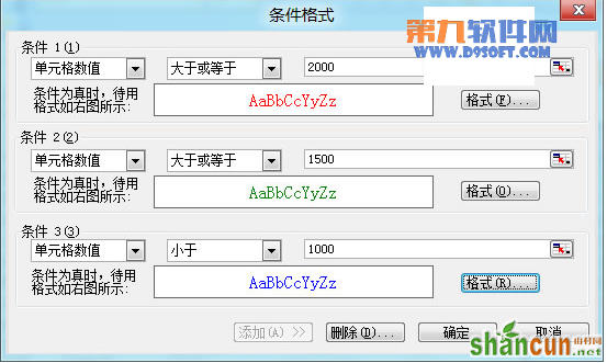
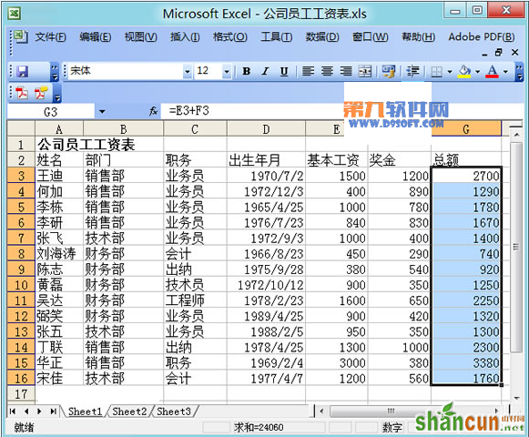
例子说明:在工资表中让大于或等于2000元的工资总额以“红色”显示,大于或等于1500元的工资总额以“绿色”显示,低于1000元的工资总额以“蓝色”显示,其它的就默认的“黑色”显示。
具体操作步骤:
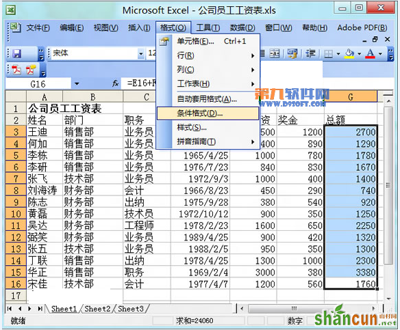
1、首先,将大于或等于2000元的工资总额设置为“红色”。选中所有员工的“工资总额”;
2、单击菜单栏的“格式”选择“条件格式”命令;
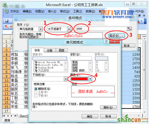
3、在弹出的“条件格式”对话框中单击第二个方框旁边的下拉按钮,设置为“大于或等于”,在后面方框中输入“2000”,然后单击“格式”按钮,在弹出的“单元格格式”中将字体颜色设为“红色”最后确定!
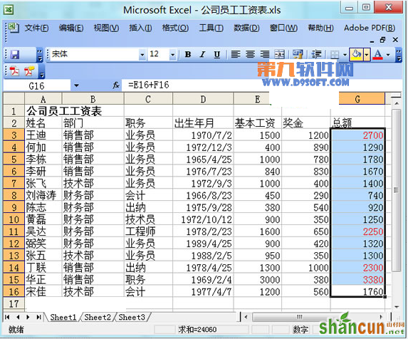
4、这里大于或等于2000元工资总额就全部变成“红色”数据了。
5、将大于或等于1500元工资总额设置为“绿色”。再次进入“格式”-->条件格式,单击“添加”按钮,在第二个方框中选择“大于或等于”,在后面方框设置1500,单击“格式”给数据字体颜色设置为绿色,最后确定。

6、此时,大于或等于1500元的工资总额数据全部变成“绿色”了。

7、下面我们来将低于1000元的工资总额设置成“蓝色”的。步骤和上面一样,进入菜单栏的“格式”选择“条件格式”。在弹出的“条件格式”中单击“添加”,然后在第二个方框中选择“小于”,在后面方框设置1000,单击“格式”给数据字体颜色设置为蓝色,最后确定即可。

提示
其实上述步骤可以更加简单一点,直接单击“格式”进入“条件格式”,一次性多添加两个条件,然后填写数据最后确定就OK了。多些步骤是希望大家更容易了解和掌握!