1、启动Excel2013,首先打开先前准备好了的数据表源,我们构建一列辅助列,判断汇总数据与达标标准的大小,看看是否达标。
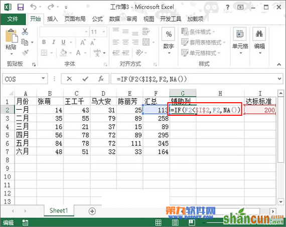
2、公式输入完毕,回车,得到结果是113,双击单元格填充柄,将数据填充完整。按住Ctrl键选中A1:A7,F1:G7区域。
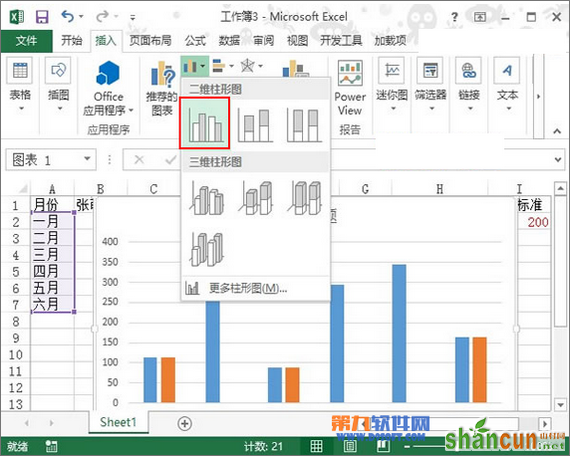
3、单击菜单栏--插入--图表,选择柱形图中的簇状柱形图。
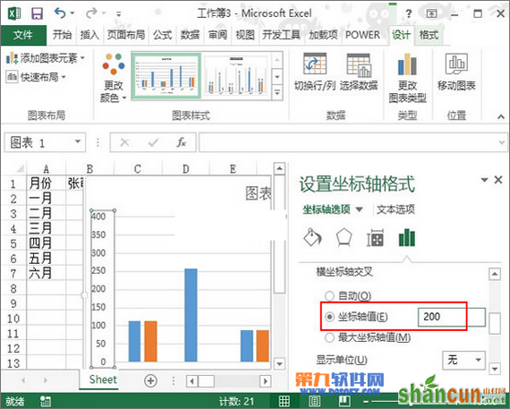
4、鼠标右键单击纵坐标轴,从弹出的右键菜单中选择设置坐标轴格式。
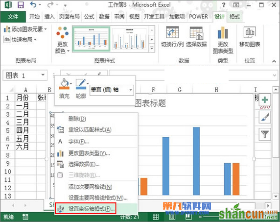
5、弹出设置坐标轴格式窗格,下拉滚动条,将横坐标轴交叉设置为200.
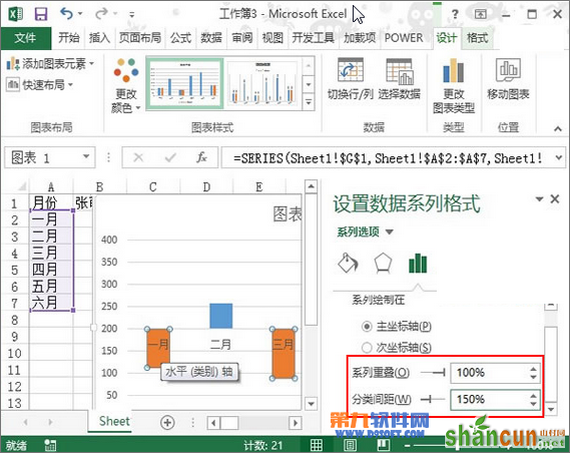
6、然后单击图表中的橙色柱形,会出现设置数据系列格式窗格,将系列重叠设置为100%,分类间距设置为150%。
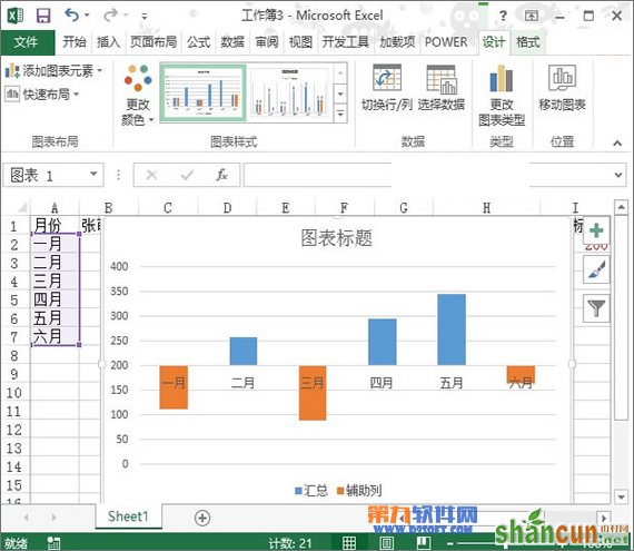
7、完成,大家可以对图表进行美化处理,删除一些不必要的东西,最后,达标图就制作完成了。图中蓝色表示达标,橙色为不达标。