使用Excel实现自动到期提醒的方法
下面讲述做一个智能的银行存款到期提醒功能。
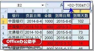
原表:
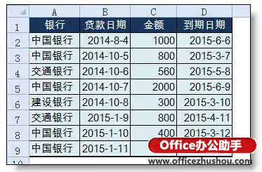
要求:
离到期日30天内行填充红色,60天内填充黄色。
效果:
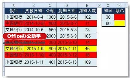
还可以修改G2:G3的期间,提醒色会自动更新
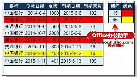
怎么样?很好玩,也很实用吧。
操作步骤:
步骤1、添加到期天数列,计算出离还款还有多少天。
公式 =D2-TODAY()
步骤2、添加辅助表,可以用来动态调整提醒的天数。
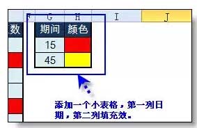
15表示15天内,45表示45天内。
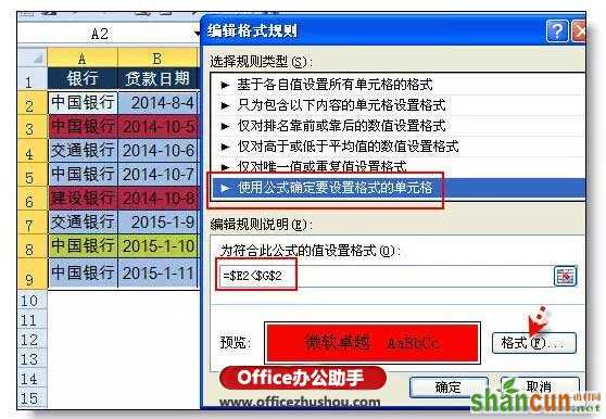
步骤3、选取表格(标题行不选),开始 - 条件格式 - 新建规则。然后进行如下设置:
类型:使用公式确定.......
设置格式框中输入公式 =$E2<$G$2(按E列到期日判断,所在E前要加$)
点格式按钮,设置填充色为红色。
步骤4、按步骤3方法,再添加一个规则。公式为=$E2<$G$3,格式设置为黄色。
步骤5、开始 - 条件格式 - 管理规则,在规则管理窗口中,把30天内规则提升到最上面。
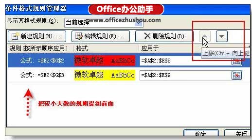
设置完成!
补充:条件格式的公式设置一定要注意,一不小心就出错。公式中引用单元格地址和引用方式同学们要看清楚了。