excel表格中怎么统计符合条件数据的和?
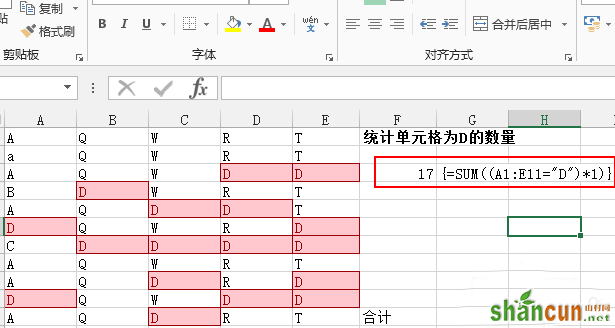
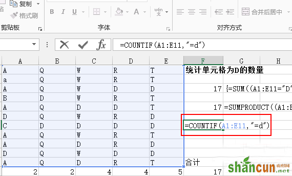
1、这里依旧使用上次的表格,可以看到已经标记的区域,我们将对这些区域统计,最最常用的函数sum,在这时可以写为”=SUM((A1:E11="D")*1)“,然后按ctrl+shift+enter进行数组运算
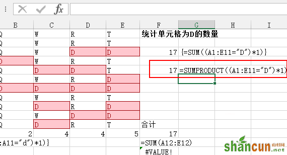
2、如果熟悉其他的函数的话,我们也可以使用sumproduct函数,如图所示。输入”=SUMPRODUCT((A1:E11="D")*1)“,直接得到结果,无需组合键
3、、还可以使用countif函数,在单元格里面输入”=COUNTIF(A1:E11,"=d")“
4、、既然countif可以使用,我们完全可以使用countifs来统计,在后面的单元格里面输入=COUNTIFS(A1:E11,"D"),不过感觉countifs用在这里有些大材小用了

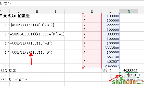
5、事实上,实际中遇到的更多的是下图中的这种表格,计算区域和条件区域泾渭分明,我们可以使用sumif函数来处理,将条件和统计区域区分。输入”=SUMIF(K1:K12,"d",L1:L12)“,其中K1:K12为条件区域,L1:L12为计算求和区域
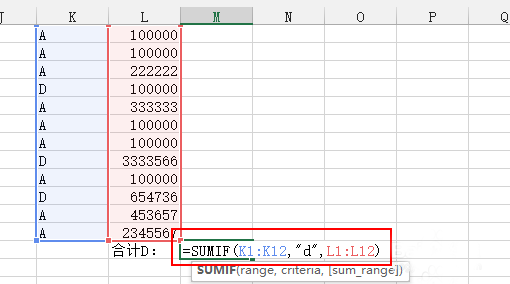
6、喜欢用sumifs的童鞋也可以在这里使用,不过需要注意统计区域和条件区域的位置和sumif的位置正好相反,判断条件放在最后,在单元格里面输入”=SUMIFS(L1:L12,K1:K12,"D")“