excel透视表制作步骤如下:
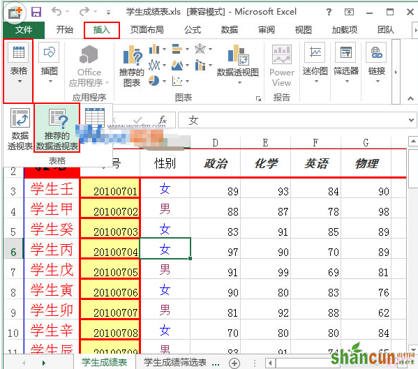
1、用Excel2013打开一篇工作表,切换到“插入”选项卡,单击“表格”组中的“推荐的数据透视表”按钮。
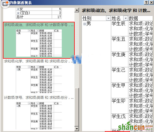
2、此时会弹出一个“推荐的数据透视表”窗口,我们在左侧的类型中根据需要选择一个数据透视表,右侧有它对应的效果,然后单击“确定”按钮。
3、返回到Excel中,我们看到窗口右侧多出了一个“数据透视表字段”窗格,大家可以在其中选择要添加到数据透视表中的字段,完成之后单击“关闭”按钮关闭窗格。
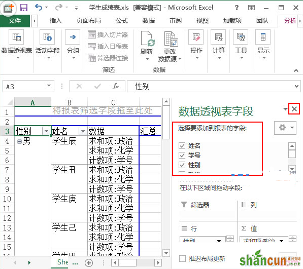
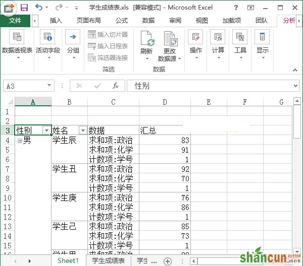
4、大家现在就能看到数据透视表的模样了,并且Excel已经自动切换到了“数据透视表工具->分析”选项卡,大家可以自己研究看看。