excel表格制作查询系统的教程:
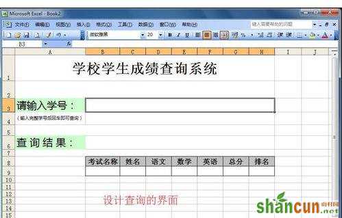
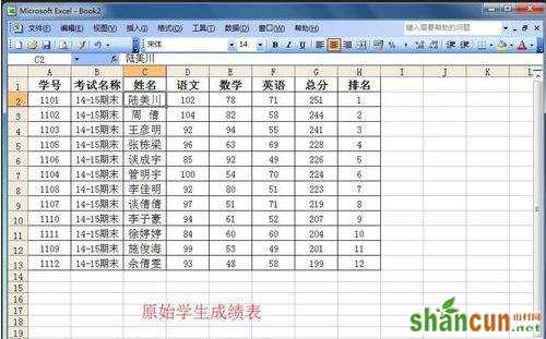
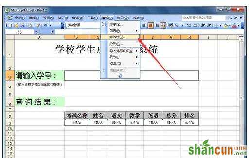
制作查询系统步骤1:首先来看一下小编设计的查询界面如图所示。学生成绩表的原始数据在sheet2工作表中。小编这里就选了12名同学成绩作为示例。
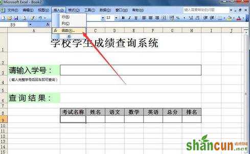
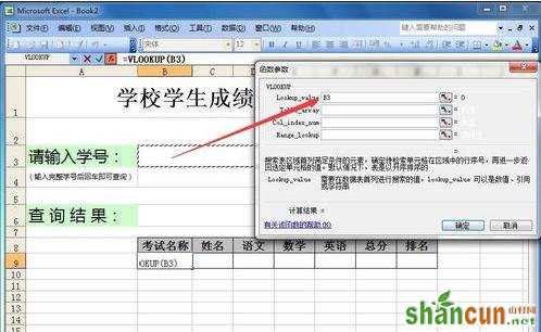
制作查询系统步骤2:单击选中B9单元格,依次单击“插入”--“函数…”。
制作查询系统步骤3:在“全部”函数中找到“vlookup”,单击“确定”按钮。红圈中提示该函数的功能(对于该函数还不太了解的童鞋可以参看小编的有关vlookup函数的经验)。
制作查询系统步骤4:第一个参数“Lookup_value”处我们单击“B3”单元格,当然也可以直接输入“B3”。
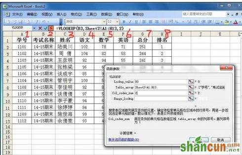
制作查询系统步骤5:第二个参数“Table_array”,我们单击sheet2工作表,选中数据区域,如图所示。
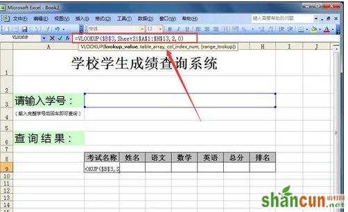
制作查询系统步骤6:第三个参数“Col_index_num”,这是满足条件单元格的列序号,我们这里要查询考试名称,当然填“2”,即第二列。其它字段的列序号如图所示。
制作查询系统步骤7:第四个参数是“Range_lookup”,即要求精确匹配还是模糊匹配。这里我们填“0”,要求精确匹配。
制作查询系统步骤8:单击“确定”以后,我们对函数修改一下,如图中红框处所示。这样修改便于我们后面的函数填充。
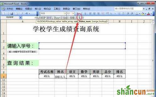
制作查询系统步骤9:修改好了直接回车,然后用填充柄直接填充函数。后面我们做一些小的修改。比如,要查询“姓名”,当然是第三列,所以这里修改为3即可。
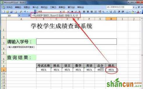
制作查询系统步骤10:以此类推,修改其它字段的函数。例如排名处我们修改函数如图中红框处所示即可。
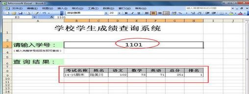
制作查询系统步骤11:测试一下,输入学号1101,回车后,查询结果全部返回正确,即我们的函数使用正确。
制作查询系统步骤12:下面我们对输入的学号进行约束。单击B2单元格,依次单击“数据”--“有效性…”。
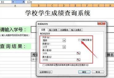
制作查询系统步骤13:第一个“设置”选项卡填写如图所示。注意:“忽略空值”取消勾选。
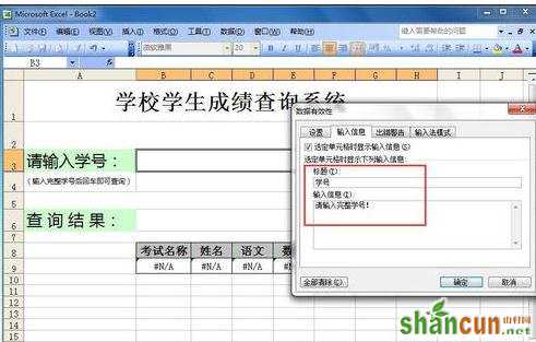
制作查询系统步骤14:第二个“输入信息”选项卡填写如图所示。
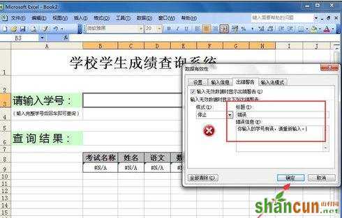
制作查询系统步骤15:第三个“出错警告”选项卡填写如图所示。至此完成输入学号的约束。单击“确定”按钮。
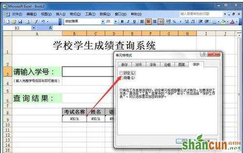
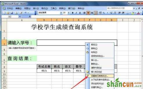
制作查询系统步骤16:然后我们对工作表进行保护,防止数据被修改。即除了B2单元格可以输入,其它单元格禁止输入或修改。右击B2单元格,选择“设置单元格格式…”。
制作查询系统步骤17:在“保护”选项卡下把“锁定”取消勾选,如图所示。
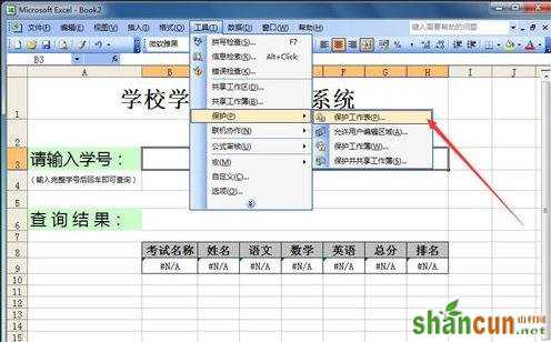
制作查询系统步骤18:依次单击“工具”--“保护”--“保护工作表…”。
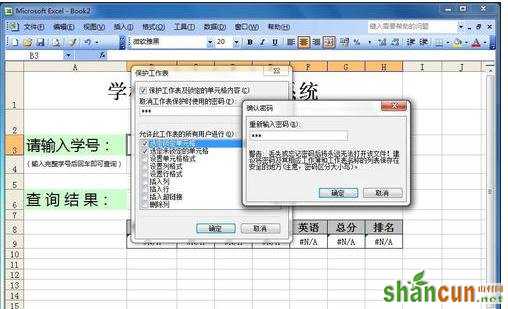
制作查询系统步骤19:输入2次密码(也可以不设置密码),单击“确定”按钮。
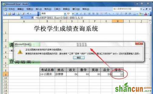
制作查询系统步骤20:这时,如果你要修改其它单元格,会弹出警告提示,如图所示。
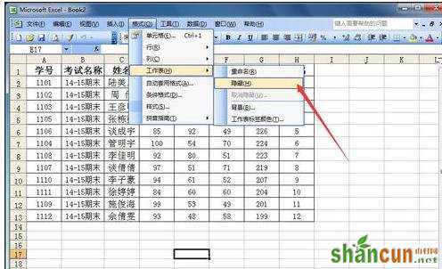
制作查询系统步骤21:为了防止原始学生成绩表受到修改,你可以把sheet2工作保护起来。也可以隐藏工作表。隐藏的方法是:在sheet2工作表中,依次单击“格式”--“工作表”--“隐藏”。如果要取消隐藏,也是在这里找到“取消隐藏”,再找到隐藏的工作表,确定即可。