图如其名,瀑布图是指通过巧妙的设置,使图表中数据点的排列形状看似瀑布悬空。这种效果的图形能够在反映数据在不同时期或受不同因素影响的程度及结果,还可以直观的反映出数据的增减变化,在工作表中非常有实用价值。以下图所示数据为例,一起学习一下如何制作瀑布图。
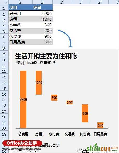
首先,来观察一下上面这个图的效果:上半部分是着色的,而下半部分是透明的。或许想到了,这样的图表应该是用到了不同的数据系列,通过对不同系列的颜色设置来实现数据系列的悬空效果。
制作瀑布图的具体操作方法如下:
1、准备数据
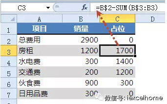
在C列增加一个“占位”的辅助列。
C2单元格写入0,C3单元格写入公式
=B$2-SUM(B$3:B3)
向下复制。
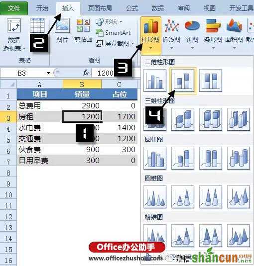
2、创建图表
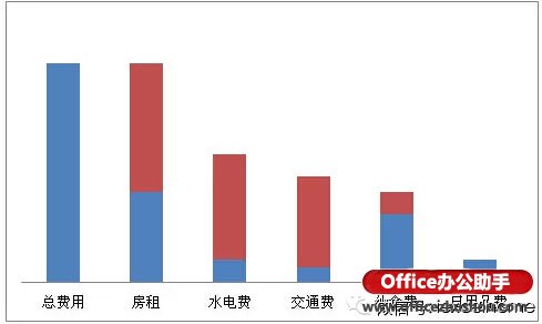
点击数据区域的任意单元格,【插入】【柱形图】选择【堆积柱形图】
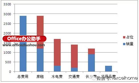
插入堆积柱形图后的效果如下:
3、清除不需要的项
依次单击图例,按Delete键删除;单击网格线,按Delete键删除;单击纵坐标轴,按Delete键删除。效果如下:
右键单击横坐标轴,【设置坐标轴格式】主要刻度线类型选择【无】
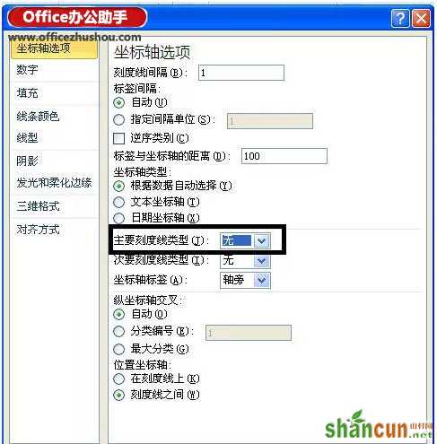
设置后的效果如下:
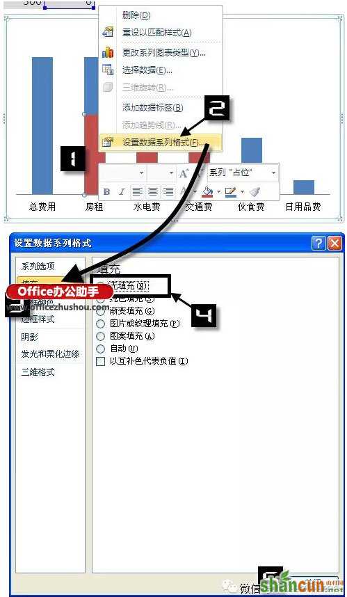
4、设置系列格式
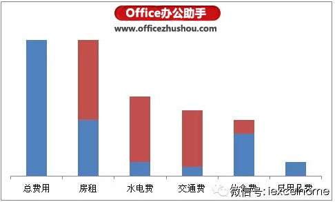
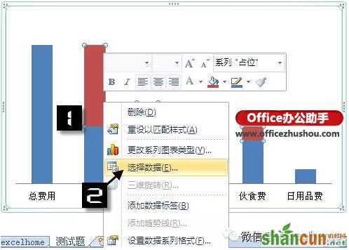
右键单击“占位”系列,【选择数据】在【选择数据源】对话框中调整数据系列的顺序,将“占位”数据系列调整到上层。
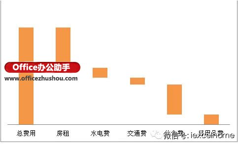
右键单击“占位”系列,【设置系列格式】【填充】选择【无填充】
参照上述步骤,右键单击“销量”系列,【设置数据系列格式】【填充】【纯色填充】选择橙色。设置后的效果如下:
5、美化图表
右键单击“销量”数据系列,添加数据标签。单击绘图区,【布局】【图表标题】【图表上方】添加图表标题。
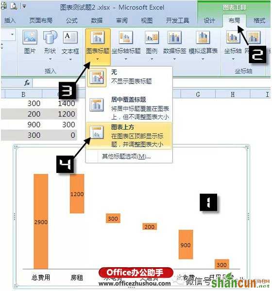
最后设置图表标题的字体,给出数据来源和制作者的信息,完成瀑布图的制作。