相信好多朋友对Excel的数据透视表的强大功能都赞叹不已。本文讲述使用Excel的数据透视表快速实现对销售员的业绩汇总、业绩占比和业绩排名的方法。
下图中,是某单位销售流水记录。
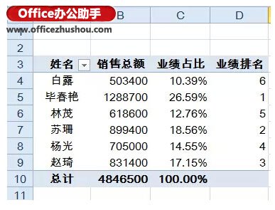
现在需要快速汇总出每个销售员的个人完成总额、销售业绩占比以及销售业绩排名,效果如下:
操作步骤:
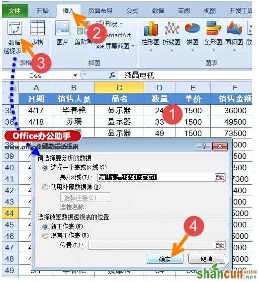
这样就在新工作表内插入一个数据透视表。
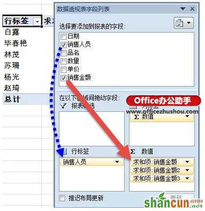
在数据透视表字段列表中,将销售人员字段拖动到行标签,将销售金额字段拖动3次到值区域。
关闭数据透视表字段列表。
右键单击销售金额2字段,设置值显示方式为“父行汇总的百分比”。
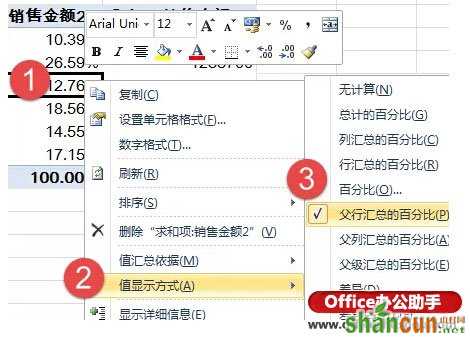
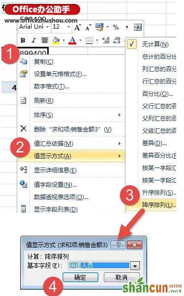
右键单击销售金额3字段,设置值显示方式为“降序排列”。
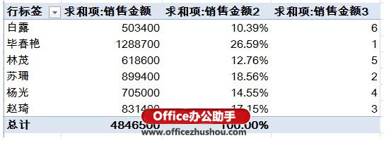
此时的数据透视表变成下面的效果:
最后修改一下字段标题:
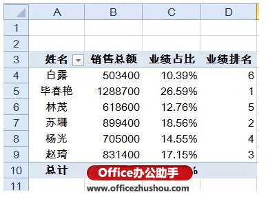
OK,已经完成了销售员的个人完成总额、销售业绩占比以及销售业绩排名。