excel制作考勤表的步骤
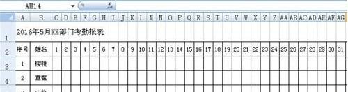
1、打开excel表格,分别输入考勤报表所需要内容:
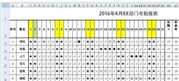
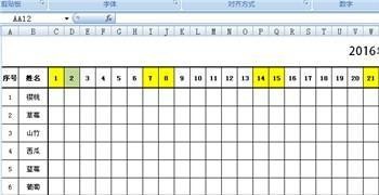
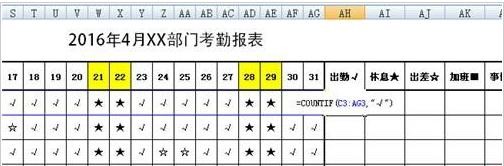
表格标题:年月+公司/部门名称+考勤报表,如2016年4月某部门考勤报表;
表格基本信息:序号、员工姓名、日期(月份不同,日期差异1~2天);
考勤考核项目:出勤、休息、出差、加班、事假、病假、婚假、产假、年假、旷工(每个考核项目均用一个符号作标识,以方便统计,考核数值的单位为天);

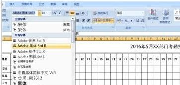
2、表格标题通过选择字体、字号、对齐方式、行高、列宽、表格边框、合并单元格等操作来实现表格美化的目的。表格美观了,工作起来不会太累。
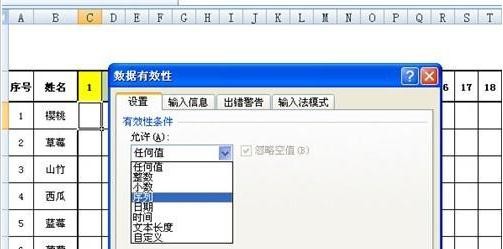
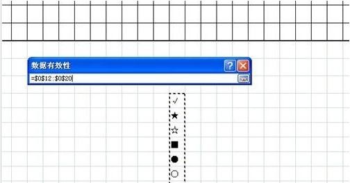
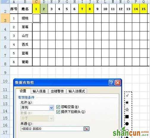
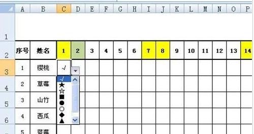
3、在表格空白处,将考勤各项目对应的符号列出来。然后,选中C3,点击【数据】-【数据有效性】,在弹出的对话框中,允许下选择【序列】,数据源选择列出来的考勤项目符号,按【回车/enter】-【确定】,即可看到C3的下拉菜单显示出考勤项目符号。
4、在AH3中输入公式:=countif(C3:AG3,"√"),按【回车/enter】。其中countif函数为对既定范围内的内容中选择出符合指定事项的求和,图例中C3:AG3是统计1~31日的符合特定选项的数值范围(注意这个范围是固定的),√为出勤项目标识符号。以此类推,用同样的公式设置考核项目,只需要将√符号替代成其他考核项目符号即可,特别注意C3:AG3是固定范围不变。设置公式完成后,直接填充下拉即可。
5、表格公式设置完成后,按员工实际上下班打卡记录,输入到表格当中,即可看到考勤考核项目统计数值会随着打卡的实际情况而有所变化。考勤统计完成后,检查无误,此项工作就圆满完成了。