excel表格底纹设置步骤:
1、选中需要添加底纹的单元格区域,单击“开始”选项卡下的“字体”组中的功能扩展按钮,如图1所示。
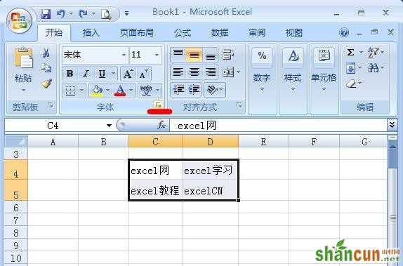
图1
2、弹出的“设置单元格格式”对话框,切换到“填充”选项卡下,在“背景色”颜色面板中选择要填充的颜色选项,如图2所示。
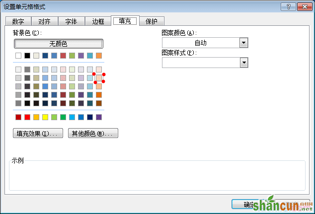
图2
3、在“图案颜色”下拉列表框中选择“橙色”选项,在“图案样式”下拉列表框中选择“细对角线平面线”选项,单击“确定”按钮,如图3所示。
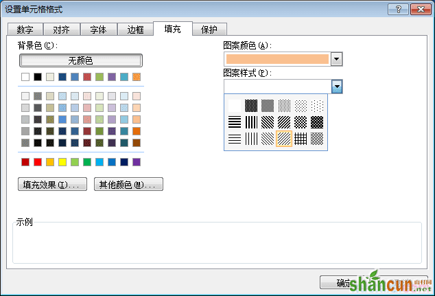
图3
4、返回到excel工作表区域,即可查看单元格区域中设置的底纹,选中其他单元格区域,再将打开的“设置单元格格式”对话框,切换到“填充”选项卡,单击“填充效果”按钮,如图4所示。
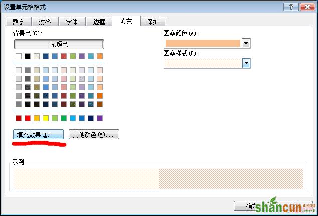
图4
5、弹出“填充效果”对话框,在“颜色1”下拉列表中选择“红色”,在“颜色2”下拉列表框右侧的下拉按钮,在其弹出的颜色面板中选择“淡红色”,如图5所示。
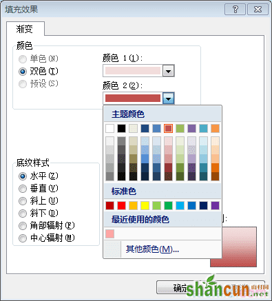
图5
6、选中“角部辐射”单选按钮,此时即可在“示例”区中查看预览效果,单击“确定”按钮,如图6所示。
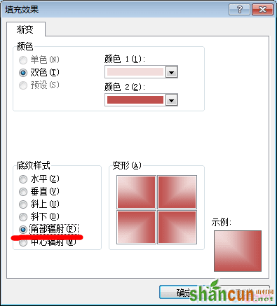
图6
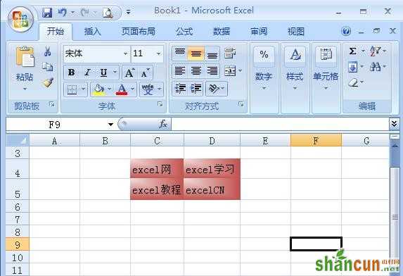
7、返回到“设置单元格格式”对话框以后,继续点击确定,然后回到工作表以后,查看效果即可,如图7所示。