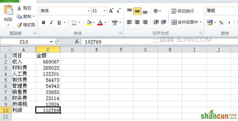
1、首先启动excel2010,执行文件-打开命令,打开事先准备好的表格数据。
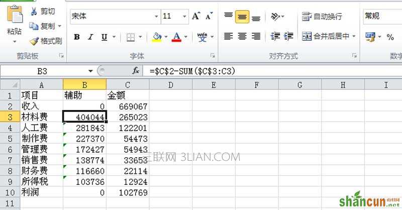
2、选择b列右键单击从下拉菜单中选择插入一列,设置标题为“辅助”,在单元格b2中输入公式=$C$2-SUM($C$3:C3),然后填充。
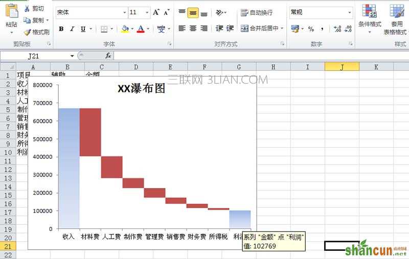
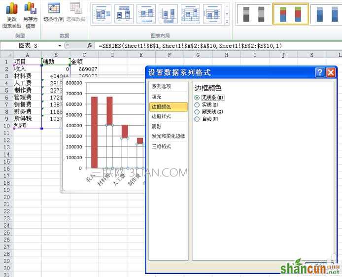
3、执行插入-柱形图命令,从下拉菜单中选择二维柱形图里的第二个椎积柱形图,这样在sheet1中就产生了一个图表。

4、右键单击蓝色柱形,从下拉菜单中选择设置数据系列格式选项,在弹出的对话框中设置填充为无填充,设置边框颜色为无线条,点击关闭按钮。
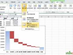
5、点击网格线选中,右键单击从下拉菜单中选择删除命令,将图表中的网格线删除。
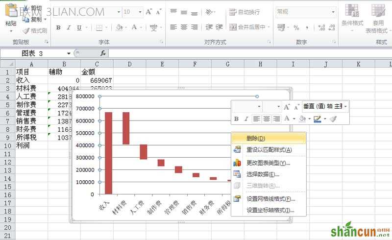
6、右键单击图表从下拉菜单中选择设置数据系列格式选项,在弹出的对话框中设置分类间距为0,点击关闭按钮。
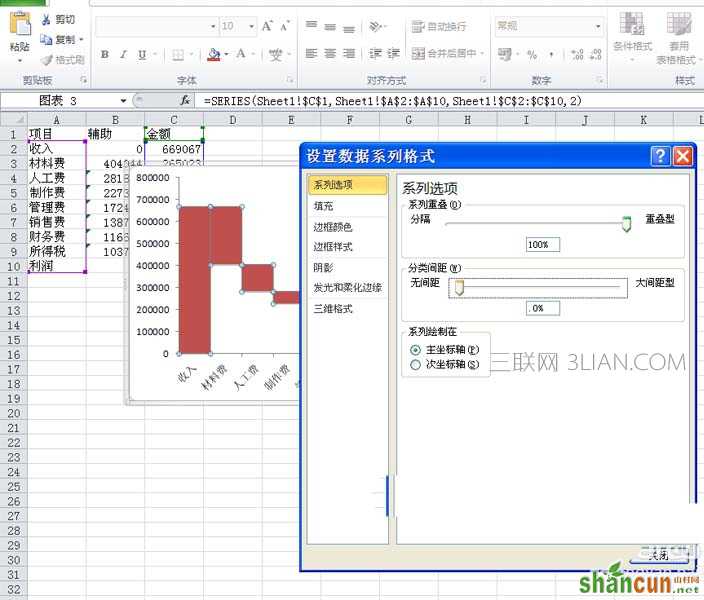
7、选择第一个柱形,右键单击从下拉菜单中选择设置数据点格式选项,在弹出的对话框中设置渐变填充,点击关闭按钮。
8、采用同样的方法将最后一个柱形进行同样的操作,接着选择图例按delete键进行删除操作。
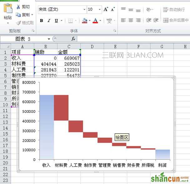
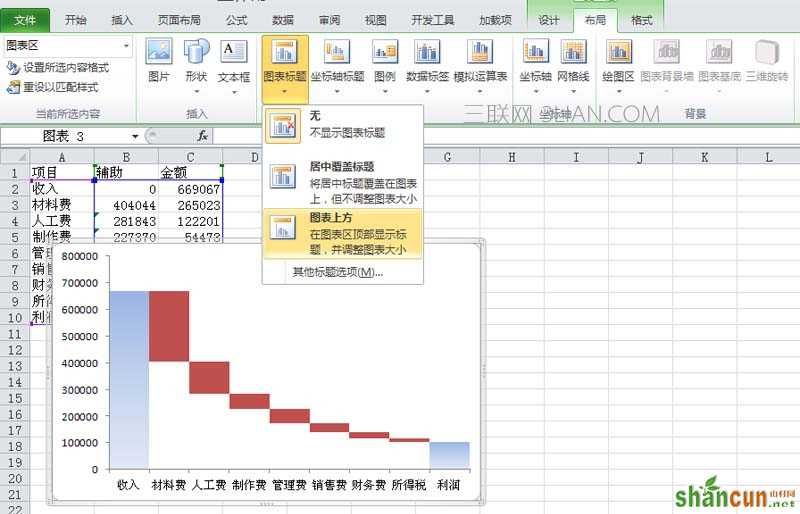
9、执行布局-图表标题命令,从下拉菜单中选择图表上方,输入标题内容“XX瀑布图”。
10、这样一个瀑布图表就制作完成了,执行文件-保存命令,在弹出的对话框中输入名称,保存在一合适的位置上即可。